Self Avoiding Walks

In my previous post titled Random Walks, I made mention of self-avoiding walks and for this post I asked Gemini 2.5 Pro to implement the following program:

Write a program in Python that will generate and display a random but self avoiding walk on a square grid of points. The size of the grid can be 100 x 100 points but this should be easily modifiable. The walk should start at the bottom left hand side and proceed to the top right hand side. Each step can be up or down from one point to the next or left or right from one point to the next but movement is contrained within the grid of points. The number of steps required to complete the walk should be prominently displayed at the top or bottom of the display.

It dutifully did this and here is the Canvas link. Here was Gemini's thinking about the desired program.

Okay, I'll provide you with a Python program that generates and displays a random self-avoiding walk on a square grid. This program uses a recursive backtracking algorithm to find a path from the bottom-left corner to the top-right corner. The grid size is easily modifiable.

Here's how the program works:

1. Grid and Path Representation: The grid is implicitly defined by its size. The path is stored as a list of (x, y) coordinate tuples.
2. Self-Avoiding Walk Generation:
   • It starts at (0,0) (bottom-left).
   • The target is (grid_size-1, grid_size-1) (top-right).
   • A recursive function attempts to find a path:
     • It marks the current cell as visited and adds it to the path.
     • If the current cell is the target, the path is found.
     • Otherwise, it randomly shuffles the possible directions (Up, Down, Left, Right).
     • For each valid direction (within bounds and not previously visited in the current path), it makes a recursive call.
     • If a recursive call returns success, the path is propagated up.
     • If all directions from the current cell lead to dead ends, it backtracks by removing the cell from the path and unmarking it as visited.
   • Due to the potential for deep recursion, especially on large grids (like 100x100), the program attempts to increase Python's recursion limit. Note that for very large grids, this process can still be computationally intensive and take some time.
3. Display:
   • matplotlib is used to visualize the walk.
   • The path is plotted on the grid.
   • Start and end points are highlighted.
   • The number of steps taken is displayed in the plot title.

I will now generate the Python code for you.

Self-Avoiding Random Walk Generator

This Python script defines two main functions: generate_self_avoiding_walk to create the path and display_walk to visualize it using matplotlib.

To use this code:

1. Save it as a Python file (e.g., saw_generator.py).
2. Make sure you have matplotlib installed (pip install matplotlib).
3. Run it from your terminal: python saw_generator.py.
4. You can easily change the GRID_SIZE variable in the if __name__ == "__main__": block to generate walks on grids of different sizes. Keep in mind that larger grids (e.g., 100x100) will take significantly longer to compute and may require a high recursion limit, which the script attempts to set.

The generated plot will show the random walk, and the title will include the number of steps taken.

I should try to implement this program myself using SageMathCell. Running the program on SageMathCell using only for a 20m x 20 grid will often cause it to time out and even in my Jupyter notebook I often needed to terminate the process because it was taking too long. However, the program often generates a walk quite quickly and Figures 1 and 2 show typical outputs.

Figure 1: permalink

Figure 2: permalink

The difference between Figures 1 and 2 in this post compared to Figure 9 in my previous post is that the latter traverses every point in the grid and not just a random selection of them. Gemini will write a program to do this but as it explains:

Finding a Hamiltonian path is an NP-complete problem. This means that for larger grids, the time required to find such a path can grow extremely rapidly. The provided recursive backtracking algorithm will explore many possibilities. For a small grid (e.g., 3x3, 4x4, maybe 5x5), it might find a solution in a reasonable time.

Here is a Canvas link to the code. Figure 3 shows a typical output using a 4 x 4 grid.

Figure 3

Probability of Two Random Integers Being Coprime

What is the probability that two integers, chosen at random, are coprime or relatively prime. In other words, they don't have any factors in common. Let's designate the random integers as \(m\) and \(n\). Let's consider a random prime \(p\). The probability that \(p\) divides \(m\) is \(1/p\) and the probability that \(p\) divides \(n\) is also \(1/p\). Therefore the probability that \(p\) will NOT divide \(m\) or \(n\) is \(1-1/p^2\). We have only considered one prime however, and need to take them all into account. So the probability that \(m\) and \(n\) have no prime factors in common is given by the following formula where \(p_i\) represents the \(p\)-th prime:$$\prod_{i=2}^{\infty} \Big (1-\frac{1}{p_i^2} \Big )= \Big (1-\frac{1}{2^2} \Big ) \Big (1-\frac{1}{3^2} \Big ) \Big ( 1-\frac{1}{5^2} \Big )\dots $$We can evaluate this using the sum of the reciprocals of all the integers squared:$$\sum_{n=1}^{\infty} \frac{1}{n^2} = 1 +\frac{1}{2^2}+\frac{1}{3^2} +\frac{1}{4^2} + \dots$$where \(n\) represents the \(n\)-th integer and where we have:$$\sum_{n=1}^{\infty} \frac{1}{n^2} \times \prod_{i=2}^{\infty} \frac{1}{p_i^2} =1$$The derivation of the above relationship is explained well in this video. However, we know that:$$\sum_{n=1}^{\infty} \frac{1}{n^2} =\zeta(2)=\frac{\pi^2}{6}$$and so$$ \begin{align} \prod_{i=2}^{\infty} \Big (1- \frac{1}{p_i^2} \Big ) &= \frac{6}{\pi^2}\\ &\approx 0.6079271 \dots \end{align}$$Thus the probability that two positive integers chosen at random are coprime is about 61%. It's easy to simulate this on a computer to test out its validity (permalink). See Figure 1.

Figure 1

Random Fibonacci Numbers

I just finished watching the latest Numberphile video on YouTube titled Random Fibonacci Numbers:

To produce these random Fibonacci numbers, what happens is that the previous two members of the sequence are added (as in the normal sequence) OR subtracted (the smaller from the larger) RANDOMLY. 

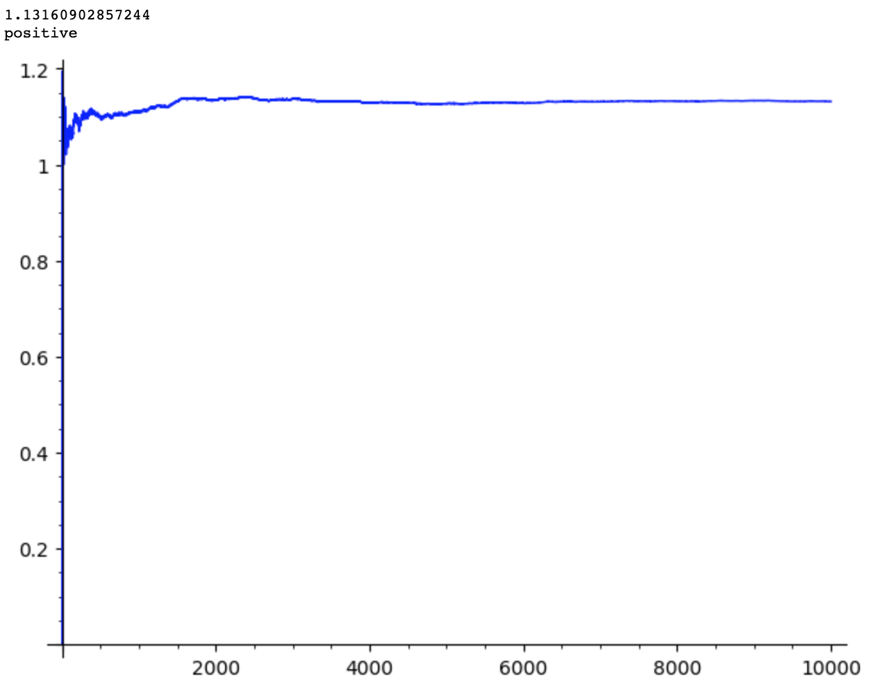
In the case of the normal Fibonacci sequence, we know that the \(n\)-th root of the \(n\)-th term approaches the golden ratio (1.6180339887…). In the randomised Fibonacci sequence, the \(n\)-th root of the \(n\)-th term approaches 1.319882487943… and this is as accurate as can currently be determined. Interestingly, as \(n\) gets larger, the \(n\)-th term can be a very large positive OR negative number. The SageMath code shown in Figure 1 calculates for 1000 terms and determines positivity or negativity:

Figure 1

Figure 2 shows an example of typical output:

Figure 2

As shown in Figure 3, a simple modification of the code , so that \(a\) must be zero, produces the standard Fibonacci sequence. 

Figure 3

Figure 4 shows an example of typical output:

Figure 4

Now in the normal Fibonacci sequence, the ratio of successive terms approaches \( \phi \) but that doesn't really work for the random Fibonacci sequence which is why the \(n\)-th root of the \(n\)-th term was chosen instead. This gets a little technical and I don't pretend to understand it but I'll quote from Wikipedia:

Johannes Kepler discovered that as \(n\) increases, the ratio of the successive terms of the Fibonacci sequence \(F_n\) approaches the golden ratio \( \phi=(1+\sqrt{5})/2\) which is approximately 1.61803. In 1765, Leonhard Euler published an explicit formula, known today as the Binet formula: $$F_n = \frac{\phi^n-(-1/\phi)^n}{\sqrt 5}$$It demonstrates that the Fibonacci numbers grow at an exponential rate equal to the golden ratio \( \phi \).

In 1960, Hillel Furstenberg and Harry Kesten showed that for a general class of random matrix products, the matrix norm grows as \( \lambda^n\), where \(n\) is the number of factors. Their results apply to a broad class of random sequence generating processes that includes the random Fibonacci sequence. As a consequence, the \(n\)-th root of |\(f_n\)| converges to a constant value almost surely, or with probability one:$$\sqrt[n]{|f_n|} \text{ --> 1.1319882487943 ...  as } n \text{ --> } \infty$$An explicit expression for this constant was found by Divakar Viswanath in 1999. It uses Furstenberg's formula for the Lyapunov exponent of a random matrix product and integration over a certain fractal measure on the Stern–Brocot tree. Moreover, Viswanath computed the numerical value above using floating point arithmetics validated by an analysis of the rounding error.

Average Distance Between Two Points in a Square

Figure 1: a unit square with vertices as shown

The problem of finding the average distance between two points in a unit square was treated in a YouTube video that I'll link to later in this post. My first response to the problem was to find to find an experimental answer by generating pairs of random points, finding the distance between them and then averaging these distances. Naturally I turned to SageMath and in particular its implementation on the Internet at SageMathCell.

Setting up an appropriate algorithm is rather straightforward given that the only formulae needed are the distance between two points and the mean. Here is the algorithm that I created and a permalink:

# (a, b) and (c, d) are random points on unit square

set_random_seed()

a, b, c, d=var('a, b, c, d')

sum, count=0,100000

for i in [1..count]:

   a=RR.random_element(0,1)

   b=RR.random_element(0,1)

   c=RR.random_element(0,1)

   d=RR.random_element(0,1)

   sum+=sqrt((a-c)^2+(b-d)^2)
print n(sum/count)

The first three results for this experiment involving 100000 points were: 

• 0.520990683987433
• 0.521024671679294
• 0.520961814850565

Clearly the exact value to close to 0.521 but what the YouTube video dealt with was a theoretical computation, leading to an exact result and not an approximate, experimental result. Here is the video and below I'll reproduce the solution (more for my own benefit as for anyone else) as it was explained there:

STEP 1: express the distance in terms of variables \(x_1\), \(x_2\), \(y_1 \) and \(y_2\)

Figure 2: application of the distance formula to two points

STEP 2: integrate the distance over the entire area $$ \int_0^1 \,  \int_0^1 \, \int_0^1 \, \int_0^1 \sqrt{(x_1-x_2)^2+(y_1-y_2)^2} \, dx_1 \, dx_2 \, dy_1 \, dy_2$$STEP 3: simplify into \(x\) and \(y\) distances and adjust for the change in probability density functions:$$ 4 \int_0^1 \, \int_0^1 \sqrt{x^2+y^2} \, (1-x)(1-y) \, dx \,dy$$\( x_1-x_2\) and \(y_1-y_2 \) collapse to \(x\) and \(y\) respectively but \(x_1\), \(x_2\), \(y_1 \) and \(y_2\) all had probably density functions of 1 e.g. \( \int_0^1 1 \, dx_1=[x]_0^1=1\). However, with \(x=|x_1-x_2| \), the probability distribution of \(x\) is given by \(2 |1-x|\) and \(2 |1-y| )\) for \(y \). This still sums to 1 because \( \int_0^1 2|1-x| \, dx =2 \times [|x-x^2/2|]_0^1=1 \). It's called a triangular probability density function. I've no idea why and at this point in time I don't understand the underlying theory, so I'm just accepting it for the moment. Later I'll try to investigate further.

STEP 4: change to polar coordinates

Figure 3: converting to polar coordinates

We make the substitutions:

\(x=r\cos \theta \) with \(0 \leq \theta \leq \pi/4 \) and
\(y=r \sin \theta \) with \( 0 \leq r \leq 1/ \cos \theta \).

Remember that the Jacobian for this change of coordinates is \(r\) and so this means that the result must be multiplied by \(r\). Integration only ranges over the lower half of the square so the integral will also need to be multiplied by 2 as well (so multiplied by 8 overall).

STEP 5: substitute the polar coordinates into the earlier integral

The new integral becomes:$$8 \int_0^{\pi/4} \, \int_0^{1/\cos \theta} \sqrt{r^2cos^2\theta + r^2sin^2 \theta} \, (1-r \, \cos \theta) \, (1-r \, \sin \theta) \, r \,dr \, d \theta$$which simplifies to:$$8 \int_0^{\pi/4} \, \int_0^{1/\cos \theta} r \, (1-r \, \cos \theta) \, (1-r \, \sin \theta) \, r \,dr \, d \theta$$which then becomes$$8 \int_0^{\pi/4} \, \int_0^{1/\cos \theta} r^2-r^3 \, \cos \theta -r^3 \sin \theta+r^4 \, \sin \theta \, \cos \theta \,dr \, d \theta$$Integrate with respect to r and substitute the limits of integration into the result.$$\int_0^{\pi/4} \bigg ( \frac{\sec^3 \theta}{12}-\frac{\sec^3 \theta \, \tan \theta}{4}-\frac{\sec^3 \theta}{4}+\frac{\sec^3 \theta \, \tan \theta}{5}\bigg ) \, d\theta $$STEP 6: solve the simplified integral

The integral can clearly be simplified into the following form:$$\int_0^{\pi/4} \bigg ( \frac{\sec^3 \theta}{12}-\frac{\sec^3 \theta \, \tan \theta}{20} \bigg ) \, d\theta$$According to the video, the result is:$$8 \bigg [\frac{ \sec \theta \, \tan \theta + \log |\sec \theta + \tan \theta \,|}{24}-\frac{\sec^3 \theta}{60} \bigg ]_0^{\pi/4}=\frac{2+\sqrt 2+5 \log (\sqrt 2 +1)}{15}$$Of course, off the cuff I wouldn't be able to carry out those integrations, so I'm just accepting them for the moment and should really try to work them out for myself. An approximation for the previous expression is 0.521405433164721 which agrees fairly closely to what I got earlier by experimentation.