Self Avoiding Walks

In my previous post titled Random Walks, I made mention of self-avoiding walks and for this post I asked Gemini 2.5 Pro to implement the following program:

Write a program in Python that will generate and display a random but self avoiding walk on a square grid of points. The size of the grid can be 100 x 100 points but this should be easily modifiable. The walk should start at the bottom left hand side and proceed to the top right hand side. Each step can be up or down from one point to the next or left or right from one point to the next but movement is contrained within the grid of points. The number of steps required to complete the walk should be prominently displayed at the top or bottom of the display.

It dutifully did this and here is the Canvas link. Here was Gemini's thinking about the desired program.

Okay, I'll provide you with a Python program that generates and displays a random self-avoiding walk on a square grid. This program uses a recursive backtracking algorithm to find a path from the bottom-left corner to the top-right corner. The grid size is easily modifiable.

Here's how the program works:

1. Grid and Path Representation: The grid is implicitly defined by its size. The path is stored as a list of (x, y) coordinate tuples.
2. Self-Avoiding Walk Generation:
   • It starts at (0,0) (bottom-left).
   • The target is (grid_size-1, grid_size-1) (top-right).
   • A recursive function attempts to find a path:
     • It marks the current cell as visited and adds it to the path.
     • If the current cell is the target, the path is found.
     • Otherwise, it randomly shuffles the possible directions (Up, Down, Left, Right).
     • For each valid direction (within bounds and not previously visited in the current path), it makes a recursive call.
     • If a recursive call returns success, the path is propagated up.
     • If all directions from the current cell lead to dead ends, it backtracks by removing the cell from the path and unmarking it as visited.
   • Due to the potential for deep recursion, especially on large grids (like 100x100), the program attempts to increase Python's recursion limit. Note that for very large grids, this process can still be computationally intensive and take some time.
3. Display:
   • matplotlib is used to visualize the walk.
   • The path is plotted on the grid.
   • Start and end points are highlighted.
   • The number of steps taken is displayed in the plot title.

I will now generate the Python code for you.

Self-Avoiding Random Walk Generator

This Python script defines two main functions: generate_self_avoiding_walk to create the path and display_walk to visualize it using matplotlib.

To use this code:

1. Save it as a Python file (e.g., saw_generator.py).
2. Make sure you have matplotlib installed (pip install matplotlib).
3. Run it from your terminal: python saw_generator.py.
4. You can easily change the GRID_SIZE variable in the if __name__ == "__main__": block to generate walks on grids of different sizes. Keep in mind that larger grids (e.g., 100x100) will take significantly longer to compute and may require a high recursion limit, which the script attempts to set.

The generated plot will show the random walk, and the title will include the number of steps taken.

I should try to implement this program myself using SageMathCell. Running the program on SageMathCell using only for a 20m x 20 grid will often cause it to time out and even in my Jupyter notebook I often needed to terminate the process because it was taking too long. However, the program often generates a walk quite quickly and Figures 1 and 2 show typical outputs.

Figure 1: permalink

Figure 2: permalink

The difference between Figures 1 and 2 in this post compared to Figure 9 in my previous post is that the latter traverses every point in the grid and not just a random selection of them. Gemini will write a program to do this but as it explains:

Finding a Hamiltonian path is an NP-complete problem. This means that for larger grids, the time required to find such a path can grow extremely rapidly. The provided recursive backtracking algorithm will explore many possibilities. For a small grid (e.g., 3x3, 4x4, maybe 5x5), it might find a solution in a reasonable time.

Here is a Canvas link to the code. Figure 3 shows a typical output using a 4 x 4 grid.

Figure 3

Hamiltonian Paths Revisited

On the 6th February 2021, I posted about Hamiltonian Paths and Knight's Tours. That was over two years ago now but today I have the opportunity to revisit the topic of Hamiltonian paths because the number associated with my diurnal age, 26996, is a member of OEIS A003778:

A003778

Number of Hamiltonian paths in \(P_5 \times P_n \).

In the case of 26996, \(n=6\).  Figure 1 shows such a \(5 \times 6 \) grid.

Figure 1

A Hamiltonian path is one that passes through every vertex exactly once. One example of such a path is shown in Figure 2. Note that in this 2D grid connections between vertices or nodes are made up-down and left-right but not diagonally.

Figure 2

In the case of a \(5 \times 6\) grid, there are 26996 such paths that can be drawn. The number of paths increases rapidly as the number of points increases. Here are the initial values:

• \(5 \times 1 \rightarrow 1\)
• \(5 \times 2 \rightarrow 22\)
• \(5 \times 3 \rightarrow 132\)
• \(5 \times 4 \rightarrow 1006\)
• \(5 \times 5 \rightarrow  4324\)
• \(5 \times 6 \rightarrow 26996\)
• \(5 \times 7 \rightarrow  109722\)
• \(5 \times 8 \rightarrow 602804\)
• \(5 \times 9 \rightarrow 2434670\) 
• \(5 \times 10 \rightarrow 12287118\)

Here is a permalink to some Python code that will plot a Hamiltonian path through a grid of specified size. Figure 3 shows the output in the case of a \(5 \times 6\) grid:

[(0, 0), (0, 1), (0, 2), (0, 3), (0, 4), (0, 5), (1, 5), (1, 4), (1, 3), (1, 2), (1, 1), (1, 0), (2, 0), (2, 1), (2, 2), (2, 3), (2, 4), (2, 5), (3, 5), (3, 4), (3, 3), (3, 2), (3, 1), (3, 0), (4, 0), (4, 1), (4, 2), (4, 3), (4, 4), (4, 5)]

Figure 3

This YouTube video does a good job of explaining in simple terms the difference between a Hamiltonian path and an Euler path. For the latter, the path must traverse every edge exactly once whereas in the former it is every vertex that must be traversed.

There is a 36-term linear recurrence mentioned in the OEIS A003778 comments which is the closest thing to a formula that seems to be available for calculating the number of possible paths. Hamiltonian paths and cycles are intimately connected with the travelling salesman problem as this site explains:

Travelling Salesman Problem (TSP): 

Given a set of cities and the distance between every pair of cities, the problem is to find the shortest possible route that visits every city exactly once and returns to the starting point. Note the difference between Hamiltonian Cycle and TSP. The Hamiltonian cycle problem is to find if there exists a tour that visits every city exactly once. Here we know that Hamiltonian Tour exists (because the graph is complete) and in fact, many such tours exist, the problem is to find a minimum weight Hamiltonian Cycle. 

Figure 4

For example, consider the graph shown in the Figure 4 on the right side. A TSP tour in the graph is 1-2-4-3-1. The cost of the tour is 10+25+30+15 which is 80. The problem is a famous NP-hard problem. There is no polynomial-time know solution for this problem. 

The site goes to provide programming solutions to this particular instance of the TSP but the Python3 solution doesn't work. However, the minimum cost Hamiltonian tour is  80 and 1-2-4-3-1 is one solution. This YouTube video offers a useful tutorial on how to draw graphs, such as the one shown in Figure 3, using SageMath.

I discovered an interesting site called Graph Online that allows you to create graphs and find Hamiltonian and Eulerian paths and cycles as well as Adjacency and Incidence Matrices. Figure 5 shows the Hamiltonian path that it came up with for the graph that I drew. No Hamiltonian cycle is possible.

Figure 5

Figure 6 shows a Eulerian path. No Eulerian cycle is possible. The site will display and analyse many other types of graphs. I've just focused on two here.

Figure 6

Hamiltonian Paths and Knight's Tours

I encountered Hamiltonian paths before but never in the context of my daily number count. The reason is clear when we look at Figure 1 showing the initial members of OEIS A003216:

A003216

Number of Hamiltonian graphs with \(n\) nodes.

Figure 1: source

Looking at Figure 1, it can be seen that \(n\)=8 yields a value of 6196 but \(n\)=9 yields a value of 177083. This is a massive jump that completely misses the numbers that I am traversing as I track my diurnal age. Currently I am 26241 days old and one of the properties of this number is that it is a member of OEIS A283420 where \(n\)=9:

A283420

Number of simple (not necessarily connected) untraceable graphs on \(n\) nodes.

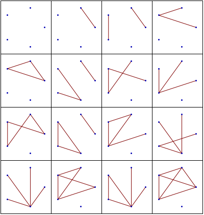
Even in the A283420 sequence the numbers get large very quickly. Here are the values from \(n\)=1 to 11: 0, 1, 2, 6, 16, 65, 310, 2316, 26241, 522596, 18766354. My current diurnal age just happened to be a member of this sequence and this is what led me to reacquaint myself with Hamiltonian graphs. Figure 2 shows all the possible non-Hamiltonian graphs for the case of \(n\)=5:

Figure 2: source

Looking at Figure 2, the distinction between graphs that are connected and those that are disconnected is apparent. But what about the terms simple and untraceable? At this point, it's a good idea to define separately what is meant by a simple graph and traceable graph (which will then explain an untraceable graph).

To quote from WolframMath World:

A simple graph, also called a strict graph, is an unweighted, undirected graph containing no graph loops or multiple edges. A simple graph may be either connected or disconnected. Figure 3 shows the differences between a simple graph and a nonsimple one:

Figure 3: source

A traceable graph is a graph that possesses a Hamiltonian path. Hamiltonian graphs are therefore traceable, but the converse is not necessarily true. The numbers of traceable graphs on \(n\)=1, 2, ... are 1, 1, 2, 5, 18, 91, 734, ... (OEIS A057864), where the singleton graph \(K_1\) is conventionally considered traceable. The first few are illustrated in Figure 4, with a Hamiltonian path indicated in orange for each. Source.

Figure 4: source

Comparing Figures 2 and 4, it can be seen what it is that defines a Hamiltonian path and a Hamiltonian cycle:

A Hamiltonian path or traceable path is a path that visits each vertex of the graph exactly once. A graph that contains a Hamiltonian path is called a traceable graph ... A Hamiltonian cycle, Hamiltonian circuit, vertex tour or graph cycle is a cycle that visits each vertex exactly once. A graph that contains a Hamiltonian cycle is called a Hamiltonian graph. Source.

Figure 5 shows a Hamiltonian cycle for the dodecahedron. 

Figure 5: source

A knight's tour can be viewed as either a Hamiltonian cycle or path when each square is regarded as a vertex:

A knight's tour is a sequence of moves of a knight on a chessboard such that the knight visits every square exactly once. If the knight ends on a square that is one knight's move from the beginning square (so that it could tour the board again immediately, following the same path), the tour is closed; otherwise, it is open. The knight's tour problem is an instance of the more general Hamiltonian path problem in graph theory. The problem of finding a closed knight's tour is similarly an instance of the Hamiltonian cycle problem. Unlike the general Hamiltonian path problem, the knight's tour problem can be solved in linear time. Source.

Figure 6 shows an open knight's tour that is a Hamiltonian path but not a cycle:

Figure 6: source

It has been shown that closed knight's tours are possible on any \(m\) x \(n\) board with \(m\) ≤ \(n\) unless one or more of these three conditions are met:

• \(m\) and \(n\) are both odd
• \(m\) = 1, 2, or 4
• \(m\) = 3 and \(n\) = 4, 6, or 8

On an 8 × 8 board, there are exactly 26,534,728,821,064 directed closed tours (i.e. two tours along the same path that travel in opposite directions are counted separately, as are rotations and reflections). The number of undirected closed tours is half this number, since every tour can be traced in reverse. Source. 

Finally let's not fail to mention the great mathematician, Sir William Rowan Hamilton, after whom the Hamiltonian paths and cycles were named. Figure 7 shows a photograph of him.

Figure 7: Hamilton (1805-1865)

For a brief account of his life, follow this link.